Accepted at NeurIPS 2026

ACD-GS: Asymmetric Curvature-aware Densification for 3D Gaussian Splatting

Houqiang Zhong1,* Tianchi Zhu1,3,* Qiang Hu2,† Xiaoyun Zhang2 Li Song1,† Wenjun Zhang1

1School of Information Science and Electronic Engineering  ·  2Cooperative Medianet Innovation Center  ·  3SJTU Paris Elite Institute of Technology
Shanghai Jiao Tong University

*Equal contribution.  †Corresponding authors.

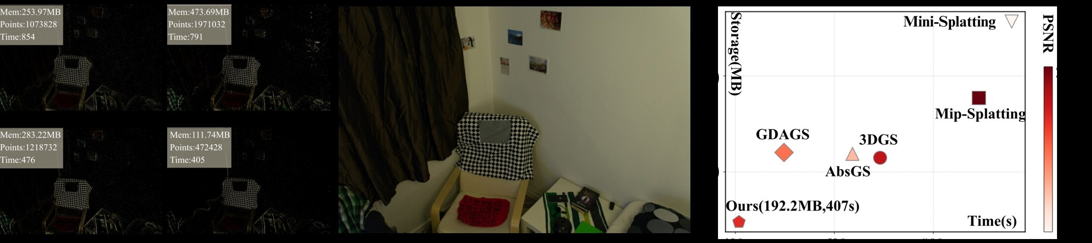
Teaser: ACD-GS point cloud comparison and storage-speed-quality trade-off

ACD-GS yields sparser Gaussians while preserving scene structure, and sits in the most favorable storage–time–quality region.

Abstract

Geometry-aware densification at its source

3D Gaussian Splatting (3DGS) has emerged as a powerful paradigm for real-time photorealistic novel view synthesis. However, its training-time densification remains largely heuristic, often resulting in redundant Gaussian proliferation and inaccurate geometric reconstruction. Existing methods predominantly rely on first-order screen-space gradients to trigger cloning and splitting, which fail to distinguish true geometric discontinuities from high-frequency textures or noisy residuals. To address this limitation, we propose ACD-GS, an Asymmetric Curvature-aware Densification framework for compact and geometry-aware 3D Gaussian optimization. Our key insight is that second-order depth responses provide a more reliable structural prior for density control, enabling asymmetric regulation of cloning and splitting to better capture geometric discontinuities. Building on this, we introduce a multi-view photometric consistency constraint to suppress transient single-view errors, together with a capacity-aware adaptive regulation strategy that balances densification and pruning during training. Unlike post-hoc compression or quantization-based approaches, ACD-GS directly prevents redundant Gaussian generation during training, yielding inherently compact representations. Extensive experiments demonstrate that our method reduces nearly 60% of Gaussian count and storage while maintaining competitive rendering fidelity, consistently outperforming existing methods across multiple datasets.

58.6% storage reduction on Deep Blending (367 MB → 152 MB)
~60% fewer Gaussians than 3DGS across all benchmarks (1.55M → 642K)
1.5–2× faster training (e.g., 683 s → 345 s on Mip-NeRF 360)
+1.1 dB PSNR over 3DGS on Deep Blending (24.03 → 25.12, best PSNR/SSIM)

Compared with the vanilla 3DGS baseline. See the paper for full per-scene results.
Method

From first-order gradients to second-order geometry priors

First-order screen-space gradients conflate flat textured surfaces, smooth slopes, and true depth discontinuities. ACD-GS instead reads the curvature of the rendered depth to build an edge-confidence map, then uses it to decouple cloning and splitting — suppressing redundant primitives at their source rather than compressing them after training.

ACD-GS pipeline overview
Overview of the ACD-GS pipeline. Click to enlarge.
1

Curvature-Guided Asymmetric Densification

A robust depth-edge confidence map E is computed from the clipped, normalized Laplacian of the rendered depth. Each visible Gaussian samples E at its projected center and receives operation-specific gradients:

giclone = gi(1 − αei)
gisplit = gi(1 + βei)

Cloning is suppressed near depth discontinuities to avoid ambiguous foreground–background duplication, while splitting is amplified so boundary-crossing Gaussians refine thin structures. In smooth regions the modulation reduces to the original 3DGS gradient, preserving texture-fitting capacity.

2

Multi-view Photometric Error Gating

Single-view residuals are volatile under occlusion and view-dependent effects. Before each densification step, K = 8 auxiliary cameras render the scene; each Gaussian is scored by the fraction of views in which its projection falls into a high-RGB-error region.

candidate  ⇔  Sirgb ≥ τmv

Only cross-view-consistent candidates enter the densification pool. This filters transient photometric noise and view-specific artifacts while still allocating capacity to genuinely under-reconstructed texture.

3

Capacity-Constrained Adaptive Optimization

Instead of a fixed gradient threshold, the densification cutoff is read from the sorted gradient distribution under a scene-aware growth quota Nallow = ⌊μNtotal⌋ (μ = 0.8%). A top-10% fallback avoids marginal candidates.

αprune(p) = αmin + (αmax − αmin) p,   p = t/T

The opacity pruning threshold is annealed with training progress: exploratory primitives survive early on, while redundant and floating Gaussians are strictly removed near convergence.

Dynamic Results

Watch Gaussians grow where geometry demands

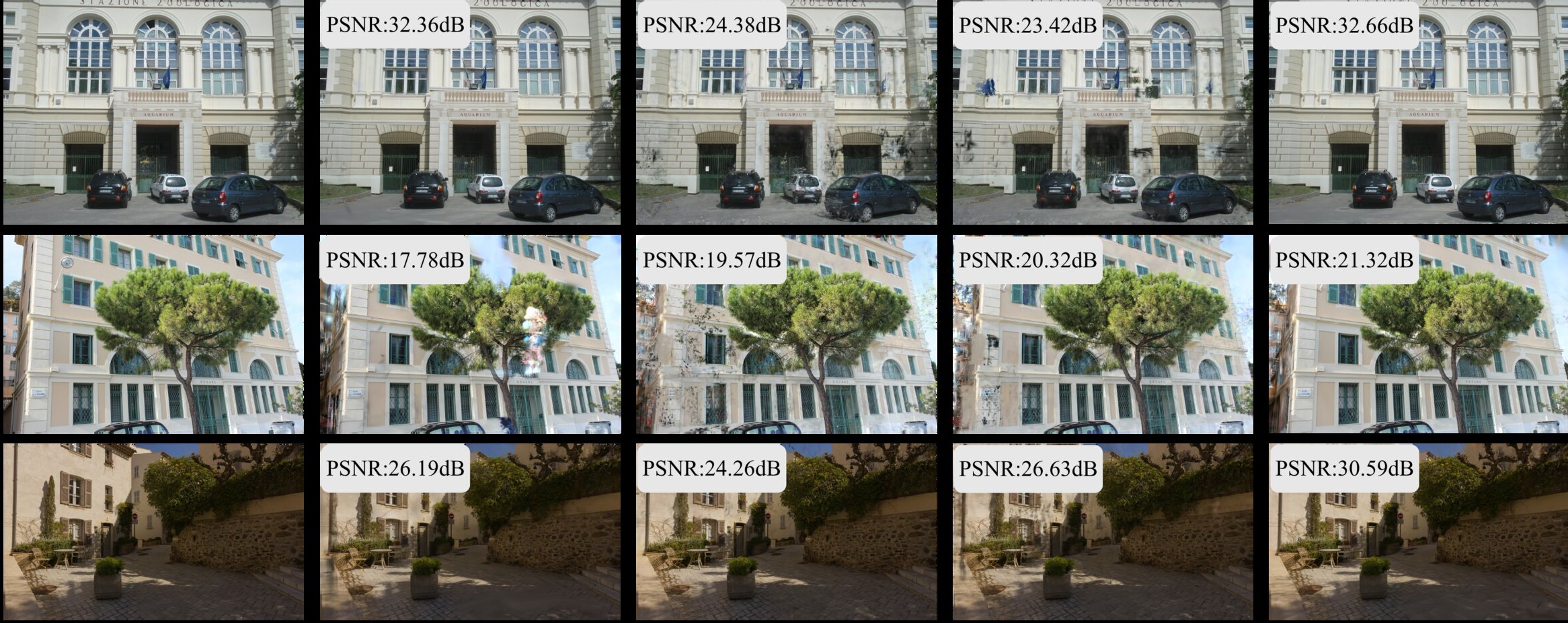
Renderings and density visualizations of ACD-GS against 3DGS and recent density-control baselines. Click a card to enlarge the image and read its caption.

Novel view synthesis comparison on Deep Blending
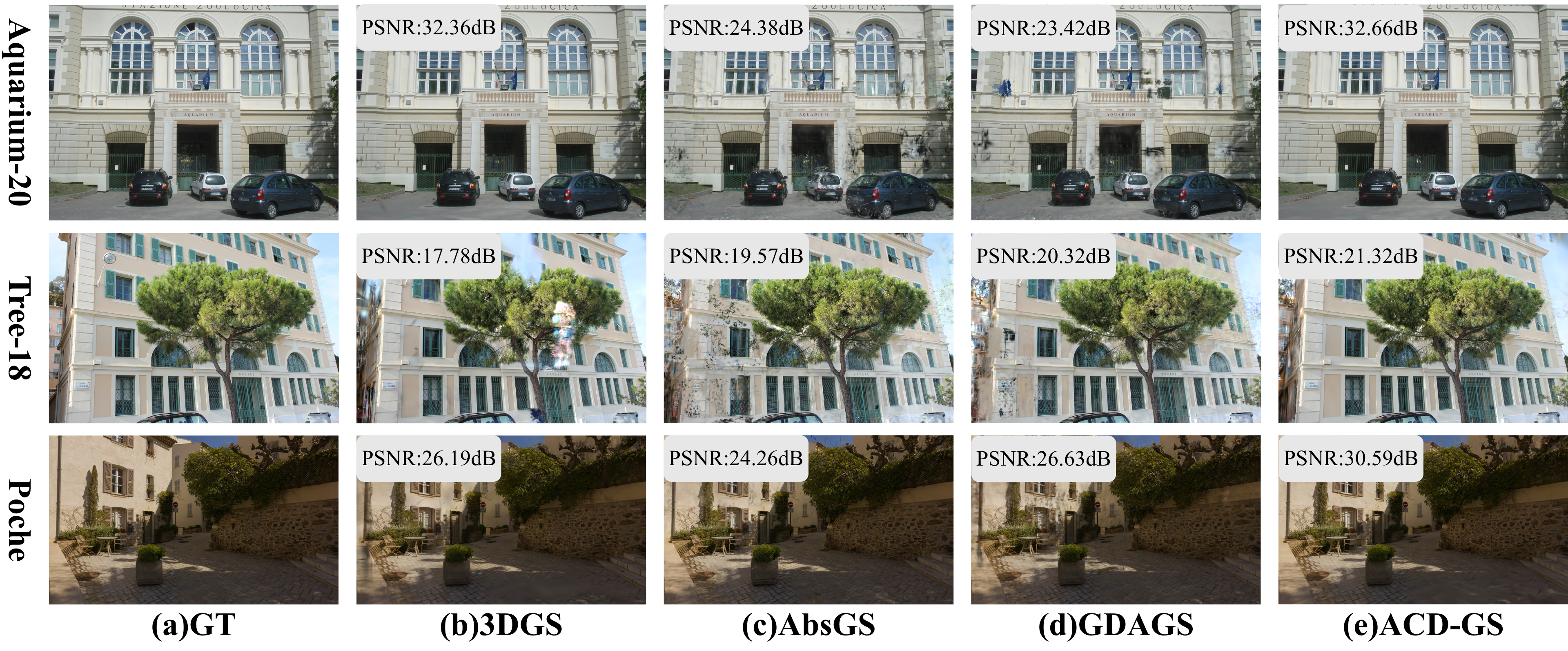
Novel view synthesis. GT vs. 3DGS vs. density-control baselines vs. ACD-GS on Deep Blending. ACD-GS removes floaters in empty regions (e.g., the sky in Tree) and keeps sharp boundaries while using a fraction of the primitives.
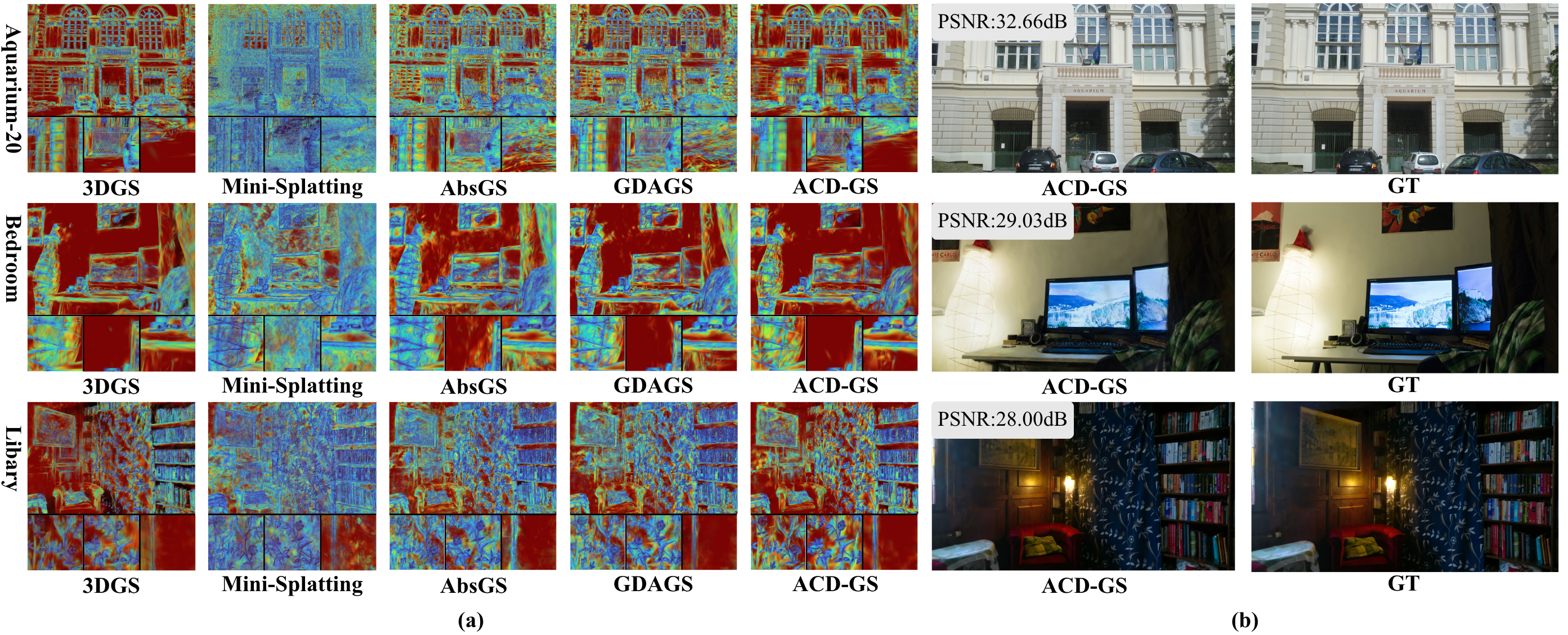
Photometric error maps and ACD-GS renders across scenes
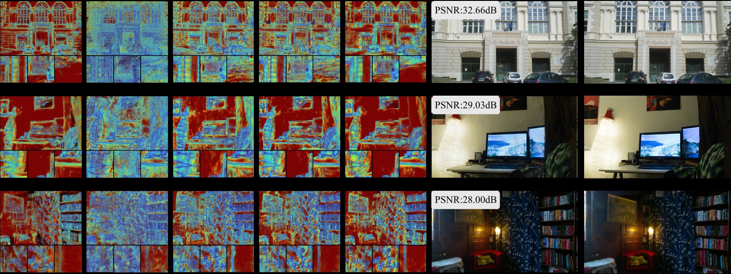
Where capacity is spent. Per-method error maps and ACD-GS renders on Aquarium, Bedroom, and Library. ACD-GS concentrates primitives along structural edges while covering planar regions with few, larger Gaussians.
Gaussian point density visualization on the Bedroom scene
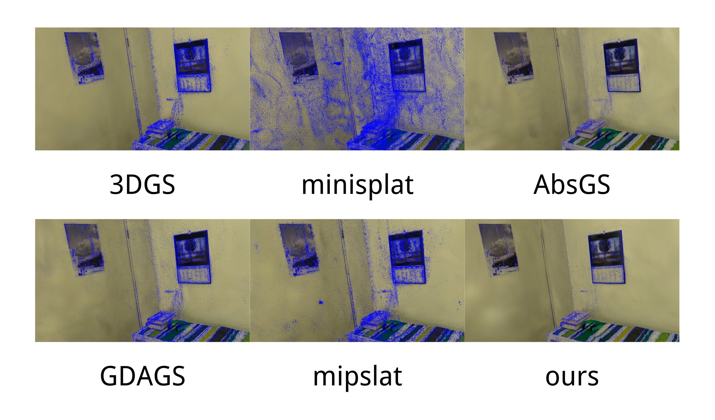
Primitive distribution. 3DGS densely saturates flat surfaces; ACD-GS allocates dense primitives strictly along structural edges and thin details, producing clean backgrounds with far fewer points.

Results

Compact models without sacrificing fidelity

Efficiency: storage, primitive count, and training time

Mean per dataset. ACD-GS uses the smallest model and trains fastest on all three benchmarks, without any post-hoc compression or quantization.

Method Deep Blending Mip-NeRF 360 Tanks & Temples
Train (s) ↓Size (MB) ↓Points ↓ Train (s) ↓Size (MB) ↓Points ↓ Train (s) ↓Size (MB) ↓Points ↓
3DGS842.0367.31.55M683.2638.42.70M551.5373.11.58M
Mip-Splatting1006.6563.22.34M955.9991.14.12M715.5569.62.37M
Mini-Splatting1125.2959.14.13M892.61108.64.69M857.01011.04.27M
AbsGS795.2400.41.69M683.2716.43.03M432.5309.41.31M
GDAGS628.1360.61.58M516.6707.12.99M350.0319.51.35M
Pixel-GS977.8694.82.94M1083.11315.15.56M945.51067.44.51M
ACD-GS (Ours)545.1151.9642.0K345.0274.31.16M333.0150.4635.7K

Rendering quality on Deep Blending (mean over 5 scenes)

MethodPSNR ↑SSIM ↑LPIPS ↓Size (MB) ↓
3DGS24.030.8310.205367.3
Mip-Splatting23.820.8220.211563.2
Mini-Splatting24.110.8240.221959.1
AbsGS23.490.7900.240400.4
GDAGS23.890.8190.215360.6
Pixel-GS24.560.8290.203694.8
ACD-GS (Ours)25.120.8340.215151.9

Best PSNR and SSIM among all compared methods, with roughly 2.4× smaller storage than 3DGS.

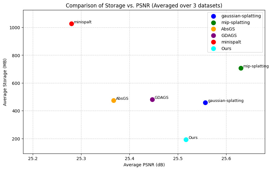
Storage vs. PSNR (averaged over 3 datasets)

Average storage versus PSNR scatter plot

ACD-GS sits in the most favorable region of the quality–compactness trade-off.

Qualitative comparison

Qualitative novel view synthesis comparison on Deep Blending
Novel view synthesis on Deep Blending. Vanilla 3DGS produces floating artifacts and texture noise; ACD-GS reconstructs clean backgrounds and crisp boundaries.
Gaussian point distribution visualization across methods
Primitive distribution: ACD-GS keeps dense primitives on structural edges and few, larger ones on planar regions.
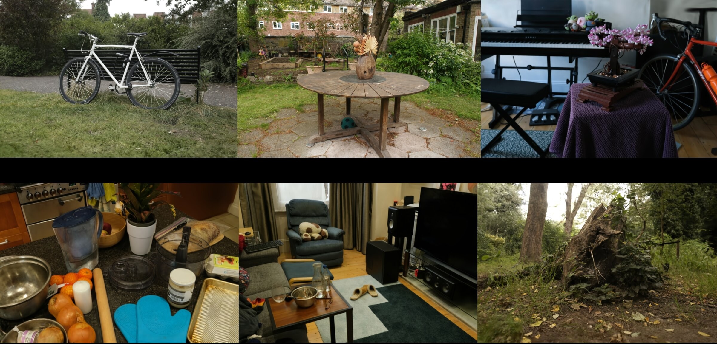
Qualitative comparison on Mip-NeRF 360
Large-scale outdoor scenes from Mip-NeRF 360.

Ablation on Deep Blending

CADMPGCAOSize (MB) ↓PSNR ↑SSIM ↑
×××360.625.220.838
✓××302.425.380.840
✓✓×159.725.380.841
✓✓✓151.925.590.845

CAD: Curvature-Guided Asymmetric Densification; MPG: Multi-view Photometric Gating; CAO: Capacity-Constrained Adaptive Optimization.

Sensitivity to α and β

SettingPSNR ↑SSIM ↑Size (MB) ↓Points ↓
α=0.5, β=1.025.310.8395247.41.05M
α=0.8, β=1.5 (default)25.590.8451151.90.64M
α=1.0, β=2.525.530.8409272.31.15M

The default setting offers the best quality–compactness trade-off.

More qualitative results

Error maps per method on three scenes
Error maps and renders on Deep Blending scenes.
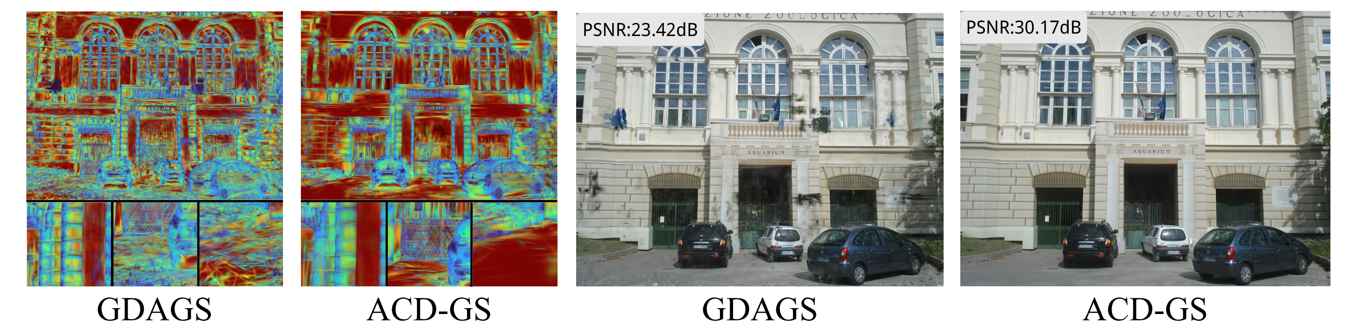
Error maps and renders of GDAGS versus ACD-GS
GDAGS vs. ACD-GS: error maps and renders. ACD-GS leaves fewer high-error residuals around geometry.

Citation

BibTeX

@inproceedings{zhong2026acdgs,
  title     = {ACD-GS: Asymmetric Curvature-aware Densification
               for 3D Gaussian Splatting},
  author    = {Zhong, Houqiang and Zhu, Tianchi and Hu, Qiang and
               Zhang, Xiaoyun and Song, Li and Zhang, Wenjun},
  booktitle = {Advances in Neural Information Processing Systems (NeurIPS)},
  year      = {2026}
}